
Text Classifier for movie reviews using Naive Bayes
- Mayukha Thumiki
- Apr 16, 2023
- 8 min read

Updated: Apr 16, 2023
Text Classification:
Using a machine learning technique, text classification involves feeding data from a text content into a set of predefined classes. However, for industrial service and government, organizations and businesses preserved their records using text documents and email. In text and document conversations, individual communication and records were also present. Due to the abundance of text information that appeared inadvertently, text classification demands have increased [1].

Objective:
This article will discuss a detailed approach of identifying the aspect of user review using Naive Bayes Theorem built from the scratch. Fundamentally, there are numerous options for categorizing Text Data, many of which are excellent at offering high levels of accuracy. However, we will examine the Naive Bayes implementation of the same in the current circumstance. The dataset for this is the rotten tomatoes movie review from kaggle contest. The collection has about 480000 items with a class type of either fresh potato or rotten tomato.
Download dataset here: https://www.kaggle.com/datasets/ulrikthygepedersen/rotten-tomatoes-reviews?resource=download
Naive Bayes Classifier:
For pattern recognition and classification that falls within several patterns of pattern classifiers for the fundamental probability and likelihood, the Naive Bayes algorithm is utilized. In earlier publications, the likelihood of such strategies was proposed. The most straightforward method of classifying texts is based on using the well-known Bayes formula. The self-determining suppositions serve as the foundation for naive Bayes approaches. With various changes, these hypotheses are obviously widely used in NLP to offer the text outline of documents and texts that are semantic, syntactic, and rational [2].
Let's delve deeper into Naive Bayes Theorem.
The fundamental assumption of the theory is naive i.e. the classes are considered as conditionally independent. This belief is referred to as "naive" since it frequently oversimplifies the reality, where aspects might be related to or dependent upon one another. Nevertheless, despite its ease of use, the Naive Bayes algorithm is widely utilized in many different disciplines, including text classification, spam filtering, and recommendation systems [3].
Math behind Naive Bayes Theorem:
The conditional probability of an event A given event B and the conditional probability of event B given event A are related by the Bayes theorem. The theorem can be expressed as follows when applied to Naive Bayes:
P(c|x) = P(x|c) * P(c) / P(x)

Source: https://www.analyticsvidhya.com/blog/2021/09/naive-bayes-algorithm-a-complete-guide-for-data-science-enthusiasts/
Where:
P(c|x) is the posterior probability of class c given the features x
P(x|c) is the likelihood probability of observing the features x given the class c
P(c) is the prior probability of class c
P(x) is the probability of observing the features x
Brief Overview of Steps followed in the Project:
Compute the prior probability of each class c. This is the probability of a randomly selected data point belonging to the class c, without considering any features.
Considering each class c, get the probable probability of detecting the traits x. This is the likelihood that the data point will include the features x if it is a member of class c.
Compute the evidence probability P(x), which is the probability of observing the features x. This probability can be computed by summing the product of the prior probability and the likelihood probability for each class.
Choose the class with the highest posterior probability as the predicted class for the data point.
Importing Libraries:
Here, we build the Naive Bayes Classifier from scratch. So, we do not require to import the inbuilt classifier. Other libraries such as nltk (Natural Language Processing Toolkit) has been used for processing purposes.

Understanding the dataset:
The below snippet discusses the loading of dataset and displaying the first 5 records. The dataset consists of sentence which is the movie review and its freshness. There are 480000 records in total.

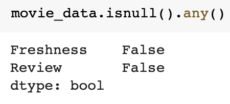
There are two classes namely 'fresh' and 'rotten' as discussed before and does not contain any missing values either.

Splitting and Processing the dataset:
This piece of code uses Pandas' replace method to replace all non-alphabetic characters in the movie_data column with spaces [4].

Using the train_test_split function from scikit-learn, this code divides a dataset into three subsets for training, testing, and validation, respectively. 80 percent of the dataset is used for training, 10 percent for validation, and 10 percent for testing [5].

Building a bag of vocabulary:
The first step is to get the count of total words as well as word frequency under each class.
Getting the frequency of all words: The function initially determines whether freshness_type is "total" or not. If not, it restricts the rows in the DataFrame df to those for which the "Freshness" column equals either "fresh" or "rotten." The function then takes every review from the filtered DataFrame and turns it into a list of words. The words are then lemmatized (or changed to their base form) using the WordNetLemmatizer from the nltk package. It only lemmatizes words that contain letters of the alphabet. The function then builds a frequency distribution object from the lemmas and returns it as a dictionary and as the FreqDist object itself [6][8].

Output after calling the fuction.

Removal of stop words: The freq_dist_list is duplicated by the function so that it can be altered while being iterated over. The function then goes over the freq_dist_list_copy iteratively and eliminates any tuple where the word is a stop word. The NLTK library's stopwords.words('english') method, which provides a list of frequent English stop words, is used to define the stop words. The function eliminates any stop words from the vocdic dictionary after removing them from the freq_dist_list. The function concludes by returning the revised vocdic dictionary and freq_dist_list [7].

Upon testing using sample data, we find that the stop words have been eliminated

Building a list of vocabulary: The code adds the lemma to the train_vocabulary list for each tuple. In essence, this function generates a list of all the distinct lemmas in the train_freq_dist_list, which can be used as a vocabulary for this model.

Marginal Probability calculation:
It is the probability of each word which is the ratio of frequency of the word to all the words in the reviews.


In the above code, wherever a value is absent, the resulting DataFrame is filled with zeros if 'st' is True. Aside from that, the DataFrame is left alone. The apply method is then used to apply a lambda function to each row of marginal_prob. Each row is normalized such that all of its values add up to 1 by the lambda function, which divides each row by the total of all of its values [8].
Training the model:
This project doesn't involve training as such. Here we calculate the likelihood probabilities of all the words. Whenever a new sentence is encountered, the model splits the data into words and searches for the likelihood probability of the word under each class. These values are multiplied and further multiplied by the prior probability of the classes. The class with high value is the predicted outcome [9].
Prior Probability calculation:
The value_counts method of the "Freshness" column of the train_data is used by the code to first determine the frequency of each class in the training data. Using the normalize=True option in the value_counts method, the obtained frequencies are then normalized to determine the likelihood of each class.

Likelihood probability calculation:
We repeat the above procedure to get the probability if words given freshness type. For this the first step is the calculation of frequency of words.

This is what the train_wfreqdf looks like.

Similar to marginal probability, we calculate likelihood as shown in the code below.


Testing using validation data:
The code first uses the split method to divide each review in the validation data into a list of words. If a word is included in the vocabulary, the code multiplies fresh_prob by the likelihood probability of the word given the "Fresh" class and rotten_prob by the likelihood probability of the word given the "Rotten" class for each word in the review. These likelihood probabilities are added to the prior probability after being taken from the likelihoodprob DataFrame. The code then adds the predicted class label ('fresh' or 'rotten') to the valid_prediction list after comparing fresh_prob and rotten_prob to determine which class is more probable [10].

Output: Generated Accuracy for Valid Data: 0.7763333333333333
Testing using Test data:
Similar procedure is followed except that the test data is used instead of valid data and we get the accuracy of about 77% for the test data.

Output: Generated Accuracy for Test Data: 0.7748958333333333
Testing using sample user given input data:

Effect of Laplacian Smoothing:
The above steps are repeated to generate a list of words including stop words, i.e. this list contains all the words in the train dataset. We then get the count of words under each category/class and find the likelihood probability of each word. Here we also increment the likelihood probability of all words by 1 so that the NaN values become incremented to one [11].
The two images show the values inside the dataframe before and after smoothing.


The below image shows the likelihood probability distribution of words after smoothing.

Upon testing using validation and test data, we get an accuracy of about 77.8% and 78.2% respectively.

Output for validation data: Generated Accuracy for Valid Data: 0.7797083333333333
Output for Test data: Generated Accuracy for Test Data: 0.7829375
Comparison of test performance before and after smoothing:
We compare the performance based on four evaluation metrics, i.e. accuracy, precision, recall and f1 score.

Graphical comparison:

Output for the above code:

Comparison using Wilcoxon:
A non-parametric statistical test called the Wilcoxon signed-rank test is used to compare two related or paired samples. When data does not adhere to a normal distribution, it is employed. The test establishes whether the median difference is 0 by comparing the differences between the paired observations. The alternative hypothesis is that there is a substantial difference, contrary to the null hypothesis, which states that there is no difference between the paired observations [12].

Deriving top 10 words that predicted each class:
We can calculate Posterior probability as
P(Class|Word) = P(Word|Class) * P(Class) / P(Word)
This can be interpreted as likelihood probability * probability_of_class / Marginal probability, while comparing the words belonging to the same class
The Bayes theory is used to determine the posterior probability of each word given that the review is either fresh or rotting as the algorithm iterates through each word in the likelihood probabilities table. The posterior probabilities for each word are then added to a new dataframe, posterior_prob. The top 10 words for each category are then obtained from the resulting dataframe, posterior_prob, which holds the posterior probabilities for each word.

Output of posterior probability of words.


The Top 10 words that predict fresh : ['cannily', 'pasi', 'ganet', 'trammell', 'protectiveness', 'enrapturing', 'elongate', 'jollied', 'raggy', 'kogonada']
The Top 10 words that predict rotten : ['revoked', 'ignominious', 'desecration', 'anthill', 'turgidly', 'ineptness', 'incurious', 'lumley', 'milling', 'overscored']
My contribution:
Removal of stop words for reducing noise and improving accuracy
Graphical and Wilcoxon comparison of performance of the model before and after smoothing
Finding the top 10 words in each class that predicted the class
Written code for naive bayes algorithm and experimented various preprocessing techniques.
Challenges:
Handling Ambiguity: The dataset has much redundant information which is not required. It has been solved by using 'replace' method and removing stop words.
Bulky dataset makes it a time taking process.
Resources:
[1] Azaria, A., Ekblaw, A., Vieira, T., & Lippman, A. (2016, August). Medrec: Using blockchain for medical data access and permission management. In 2016 2nd international conference on open and big data (OBD) (pp. 25-30). IEEE.
[2] Vijayarani, S., Ilamathi, M. J., & Nithya, M. (2015). Preprocessing techniques for text mining-an overview. International Journal of Computer Science & Communication Networks, 5(1), 7-16.
[3] Vellingiriraj, E. K., Balamurugan, M., & Balasubramanie, P. (2016, November). Information extraction and text mining of Ancient Vattezhuthu characters in historical documents using image zoning. In 2016 International Conference on Asian Language Processing (IALP) (pp. 37-40). IEEE.
[8] https://karthikvadloori.wixsite.com/home/post/text-classifier-ford-sentence-classification-using-nbc
[12] https://docs.scipy.org/doc/scipy/reference/generated/scipy.stats.wilcoxon.html
Link to code:
Colab Notebook: https://colab.research.google.com/drive/17pyBi38HYGSRsAktGQ8ZMTYzfWzJc1JY?usp=sharing


Comments