
Image Classification of Mango Leaf Disease - CNN, Decision Tree, KNN, NBC and Voting Classifier
- Mayukha Thumiki
- Apr 30, 2023
- 9 min read

Updated: Apr 30, 2023

Preface: The Indian economy heavily depends on agricultural output, yet pests and plant diseases severely impede it. In the last two decades, machine learning algorithms have made significant progress toward resolving this issue. The current systems, however, need a lot of calculation and are expensive to implement. Building a lightweight deep learning model that classifies leaf photos from a dataset of 8 classes with 3200 training images and 800 validation images is what drives this project's motivation to address all of these difficulties.
Image classification: Image classification is a computer vision task that involves assigning a label to an image based on its content. It has applications in object and facial recognition, and autonomous vehicle navigation [1]. In this article, we shall deal with image classification of mango leaf diseases by comparing the performance of different models. The majority of the time, deep CNN training was carried out using a deep learning framework [2]. To segment the disease area, some segmentation techniques also include employing Support Vector Machine (SVM), Bayes classifier, genetic algorithms, and K-means algorithm. There are further methods for spotting plant diseases that compare images with various color spaces like CIELAB, YCbCr, and HSI [3].
Project Tutorial:
The dataset for this was obtained from kaggle.
Download the dataset from: https://www.kaggle.com/datasets/aryashah2k/mango-leaf-disease-dataset
It contains 4000 Mango leaf images in JPG format with around 1800 distinct images and 2200 augmented images. There are 8 classes in total namely 'Anthracnose', 'Bacterial Canker', 'Cutting Weevil', 'Die Back', 'Gall Midge', 'Healthy', 'Powdery Mildew' and 'Sooty Mould'. Here are a few examples.

Let us begin with the project while learning simultaneously CNN, Decision Tree, Multinomial Naive Bayes, K-Nearest Neighbors and Voting classifier.
Importing Libraries
All the libraries required to perform specific tasks are mentioned in the code below. We import libraries in order to use their pre-existing functions and classes that make it easier to perform certain operations or tasks. These libraries contain pre-written code for commonly used functions that have been optimized for performance and reliability. By importing a library, we can reuse these functions in our code, rather than having to write everything from scratch, which can save us a lot of time and effort. Additionally, libraries can often provide us with powerful tools that we might not have the expertise or resources to develop ourselves.

Fetching Data
We can either use the dataset uploaded on drive or can simply fetch from the kaggle using credentials. This is comparatively less cumber some process.

The data is imported from kaggle in the format shown.

The process for preparing the dataset.


The dataset is then sampled without resetting its index and divided 20% for testing as shown.


Creating new folders
This is an optional step where we create new folders for both train and test and store the image paths in a csv format for quick and time efficient access, by performing the steps below.

The newpath variable stores the target directory path. The if statement checks if the directory already exists and creates it if it does not. The for loop iterates over each class and creates a subfolder for it in the target directory using os.makedirs(). The second for loop iterates over each image for the current class and uses shutil.copy() to copy it to the appropriate class subfolder in the target directory. Finally, the last two lines of code save the train and test DataFrames as CSV files in the current directory.
Preparation of Features and Labels for model fitting
This program loads and prepares image data for a model of machine learning. Using the Keras load_img function, it reads image files from file directories and converts them to numpy arrays using img_to_array. For the training and testing sets of data, X_train and X_test, respectively, it generates two sets of arrays. The values approach is also used to extract the corresponding labels from the train and test data. In order to make the X_train array consistent with the input shape anticipated by some machine learning models, it flattens the array into a 2D array using the reshape technique.

CNN model:
A CNN is a particular type of network design for deep learning algorithms that is utilized for tasks like image recognition and pixel data processing. Although there are other kinds of neural networks in deep learning, CNNs are the preferred network architecture for identifying and recognizing objects [4].

Parameters sharing is the technique is used by CNN. Every node in a CNN layer is connected to every other node. As the layers' filters move across the image, a CNN also has a corresponding weight; this is referred to as parameter sharing. Each layer's output, or the image that can only partially be recognized after each layer, serves as the input for the following layer. The CNN recognizes the image or object it represents in the final layer, which is an FC layer.
First we will deal with a simple CNN model that runs 5 epochs based on the training data and checks for the validation using val data which has been obtained by splitting the train data in the ratio 80:20 similar to splitting test data.


Model: "sequential" _________________________________________________________________ Layer (type) Output Shape Param # ================================================================= conv2d (Conv2D) (None, 222, 222, 32) 896 max_pooling2d (MaxPooling2D (None, 111, 111, 32) 0 ) conv2d_1 (Conv2D) (None, 109, 109, 64) 18496 max_pooling2d_1 (MaxPooling (None, 54, 54, 64) 0 2D) conv2d_2 (Conv2D) (None, 52, 52, 128) 73856 max_pooling2d_2 (MaxPooling (None, 26, 26, 128) 0 2D) flatten (Flatten) (None, 86528) 0 dense (Dense) (None, 128) 11075712 dropout (Dropout) (None, 128) 0 dense_1 (Dense) (None, 8) 1032 ================================================================= Total params: 11,169,992 Trainable params: 11,169,992 Non-trainable params: 0 _________________________________________________________________
Epochs:

Results of the CNN model are:
25/25 [==============================] - 0s 6ms/step - loss: 2.0803 - accuracy: 0.1138 Test accuracy: 0.11375000327825546

My Contribution to CNN:
I have imported the dataset using 'tf.data.Dataset' format for a better accuracy and faster data processing which I have discovered over the course of project.
The below code shows the process of splitting dataset with 80% train data and 10% each for validation and test data.

In order to improve efficiency, this code block augments the training data with random flips and rotations before prefetching it. Prior to sending the images to the neural network, it also scales and resizes them using a sequential model. Additionally defined are the input shape, the number of classes, and the number of epochs.

The model is designed using hyper parameter tuning and selecting the best parameters high model performance as shown in the code.

Output of model summary:

Model: "sequential_3" _________________________________________________________________ Layer (type) Output Shape Param # ================================================================= sequential_2 (Sequential) (32, 224, 224, 3) 0 conv2d_3 (Conv2D) (32, 222, 222, 32) 896 max_pooling2d_3 (MaxPooling (32, 111, 111, 32) 0 2D) conv2d_4 (Conv2D) (32, 109, 109, 64) 18496 max_pooling2d_4 (MaxPooling (32, 54, 54, 64) 0 2D) conv2d_5 (Conv2D) (32, 52, 52, 64) 36928 max_pooling2d_5 (MaxPooling (32, 26, 26, 64) 0 2D) conv2d_6 (Conv2D) (32, 24, 24, 64) 36928 max_pooling2d_6 (MaxPooling (32, 12, 12, 64) 0 2D) flatten_1 (Flatten) (32, 9216) 0 dropout_1 (Dropout) (32, 9216) 0 dense_2 (Dense) (32, 64) 589888 dropout_2 (Dropout) (32, 64) 0 dense_3 (Dense) (32, 8) 520 ================================================================= Total params: 683,656 Trainable params: 683,656 Non-trainable params: 0 _________________________________________________________________
Model training:

Output of the accuracy values are:
Test accuracy: [0.3540624976158142, 0.6887500286102295, 0.7774999737739563]
Validation accuracy: [0.578125, 0.8177083134651184, 0.8411458134651184]
Loss: [1.6152081489562988, 0.8135330080986023, 0.561306893825531]
Validation loss: [1.2494468688964844, 0.53177410364151, 0.4672270119190216]

Comparison of two CNN models:
This graph compares the accuracy of two models in simple line plot.

My contribution to comparison with in-built models:
1. Decision Tree: The non-parametric supervised learning approach used for classification and regression applications is the decision tree. It is organized hierarchically and has a root node, branches, internal nodes, and leaf nodes [5].

By using a greedy search to find the ideal split points inside a tree, decision tree learning uses a divide and conquer technique. The dividing procedure is then iterated upon in a top-down, recursive fashion. Pure leaf nodes, or data points belonging to a single class, are easier to obtain in smaller trees. It gets harder to preserve this purity as a tree gets bigger, which typically leads to too little data falling under a particular subtree. This is known as data fragmentation, and it frequently results in overfitting. Because of this, decision trees favor tiny trees.
The code for training using decision tree is shown below.

The results obtained upon testing are:

Training accuracy: 0.695
Test Accuracy: 0.61125
Test Precision: 0.6137127495706378
Test F1 Score: 0.6038363712830711
Test Recall: 0.609245729479907
Confusion matrix is as follows:

2. Multinomial Naive Bayes: An approach to Bayesian learning that is well-liked in Natural Language Processing (NLP) is the Multinomial Naive Bayes algorithm. Using the Bayes principle, the computer makes an educated prediction about the tag of a text, such as an email or news article. It determines the likelihood of each tag for a particular sample and outputs the tag with the highest likelihood. However, it may also be used in image classification for extracting features [6].

Source: https://insightimi.wordpress.com/2020/04/04/naive-bayes-classifier-from-scratch-with-hands-on-examples-in-r/
Each pixel in an image can be viewed as a feature when discussing image categorization. The frequency of pixel values in each image can therefore be used to classify images using the MNB method. Overall, Multinomial Naive Bayes can still be helpful for straightforward image classification tasks where computational resources are constrained, even though it may not be the best algorithm for image classification compared to more sophisticated deep learning models [7].
Code for training using multinomial NBC:

The results obtained are:

Training accuracy: 0.5203125
Test Accuracy: 0.50875
Test Precision: 0.5111100191549853
Test F1 Score: 0.5005918228776082
Test Recall: 0.5116827365909208
Confusion Matrix:

Principal component analysis (PCA): The high-dimensional feature spaces that result from the typical large number of possible pixel intensity values present a barrier when utilizing Multinomial Naive Bayes for picture classification. Principal Component Analysis (PCA), a dimensionality reduction approach, can be used to decrease the amount of features in order to get around issue. Here is an illustration.

The second line in the above code snippet creates a PCA object with 14 principal components and fits it on the flattened training images to reduce their dimensionality. Reducing the dimensionality of the training images with PCA helps to remove noise and redundancy in the data, which can lead to improved classification performance by reducing the chance of overfitting. It also helps to speed up computation by reducing the number of features that need to be processed. The number of principal components chosen, in this case 14, is typically determined by balancing the need for a reduced feature space with the desire to maintain as much information as possible.
this code creates a scatter plot of the first 14 main components produced by conducting PCA on the flattened training images, with each point colored according to its corresponding label in y_train.

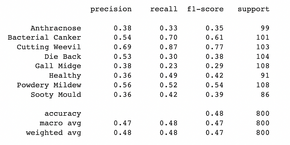
Classification report obtained upon training the model with data using 14 principal components is shown below.
Cochran's Q Test for comparing performance of models: The code performs Cochran's Q test to compare the performance of two classification models: Naive Bayes with PCA and Multinomial Naive Bayes without PCA. The contingency table is first created using the confusion matrices of the two models on the test set. A small constant value is added to the table to avoid any zero values. The p-value obtained from the Cochran's Q test is then checked against a significance level of 0.05. Since the p-value is less than or equal to 0.05, it means that at least one of the models significantly outperforms the others.

3. K-Nearest Neighbors: The k-nearest neighbors algorithm, sometimes referred to as KNN or k-NN, is a supervised learning classifier that employs proximity to produce classifications or predictions about the grouping of a single data point [8].

Source: https://towardsdatascience.com/building-a-k-nearest-neighbors-k-nn-model-with-scikit-learn-51209555453a
In the above image, a data point is taken and the nearest 'k' labeled data points are examined in k-NN models. The bulk of the 'k' closest points' labels are then applied to the data point. The data point in question would be labeled "green" since "green" is the majority (as seen in the preceding graph), for instance, if k = 5 and 3 of the points are "green" and 2 are "red".
Training using KNN

Results obtained are:

Training accuracy: 0.780625
Test Accuracy: 0.6425 Test Precision: 0.6627463204723946 Test F1 Score: 0.6390885837238719 Test Recall: 0.6434821052984503
Confusion Matrix:

4. Voting Classifier: A voting classifier is a type of machine learning estimator that develops a number of base models or estimators and makes predictions based on averaging their results. Voting for each estimator output can be integrated with the aggregating criteria [9].

How can performance be improved with voting classifier?
On the basis of hard voting or soft voting, the voting classifier accumulates the anticipated class or projected probability. Therefore, the voting classifier ensures that the error is resolved by any model if we feed it a variety of base models.
In the given code, four classifiers are defined:
tree_clf: A decision tree classifier with maximum depth of 4
nb_clf: A multinomial naive bayes classifier
ann_clf: A multilayer perceptron classifier with one hidden layer of 128 neurons, using rectified linear unit (ReLU) activation function, Adam solver and maximum number of iterations set to 100
knn_clf: A k-nearest neighbors classifier with k=5
Finally, a VotingClassifier is defined, which takes the above classifiers as inputs and uses a 'hard' voting scheme to make predictions. The VotingClassifier combines the predictions of each of the classifiers and returns the class with the highest number of votes as the final prediction.

Results are:

Training accuracy: 0.6553125
Test Accuracy: 0.58625
Test Precision: 0.6495803352573939
Test F1 Score: 0.5776819735860956
Test Recall: 0.5904961001756369
Confusion Matrix:

Visual Comparison and Analysis:
A. Comparison of train and test accuracies:

B. Comparison of different model test performances:

C. Comparison with my CNN model test performance

Result:
CNN outperforms all the other models by achieving an accuracy close to 75%, while other models have an accuracy ranging between 50% and 65% which is a significant difference. Additionally, CNNs can handle a lot of data, which makes them ideal for jobs like image classification.
My Contribution
New CNN model: Created a CNN model that accesses data using Tensorflow to simplify access and reduce complexity. In the process, DataGenerator was used for data augmentation, resized and rescaled images for improvement of performance.
Hyper parameter tuning: Models are created by fine-tuning with hyperparameters and comparing to the best accuracy that could be determined for the model. Tried epochs, batch_size, image size and number of neurons to fix the errors and losses to give best model performance
Performance Comparison: Compared the performance of five different classification models, visualizing each one separately and in a subplot side by side to understand how accurate each model was for each kind of class label.
Data Visualization: Confusion Matrix is included to each model after prediction is complete in order to determine the truth value of the minimal correlation between classes and to support the validity of the accuracy produced.
Principal Component Analysis: Performed PCA for multinomial Naive Bayes and performed Cochran's Q Test for comparing performance of models
Challenges:
Time complexity: Training time for CNN model by accessing data using image paths was too high. Hence, I accessed the dataset in tensorflow format which not only gave faster but more accurate results. Also,since Scikit-learn models cannot accept Image Data Iterator types as input, I had trouble making the prediction and had to separately encode an images and labels list object by passing the image and appending it to them.
Overfitting: I had overcome the problem of overfitting in all the models by hyper parameter tuning
Complexity due to high dimension data: Using Multinomial Naive Bayes for classification in high-dimensional feature spaces of images might be difficult. To solve this problem, dimensionality reduction methods, i.e., PCA was used.
Link to code:
Colab Notebook: https://colab.research.google.com/drive/1SF0T2tBdgCj2Vi8_6_neCFyq0j_pV3qo?usp=sharing
Kaggle Notebook:
https://www.kaggle.com/code/thumikimayukha/mango-leaf-disease-classification/notebook Github Link:
https://github.com/mayukhathumiki876/Maongo-Leaf-Disease-Image-Classification/blob/982656df7d4c25f15ab672905901c1a6f012fb39/Main_Project.ipynb
Link to dataset:
References:
[1] Syarief, M., & Setiawan, W. (2020). Convolutional neural network for maize leaf disease image classification. Telkomnika (Telecommunication Computing Electronics and Control), 18(3), 1376-1381.
[2] Chakraborty, A., Kumer, D., & Deeba, K. (2021, April). Plant leaf disease recognition using fastai image classification. In 2021 5th International Conference on Computing Methodologies and Communication (ICCMC) (pp. 1624-1630). IEEE.
[3] Piyush Chaudhary, Anand K. Chaudhari, Dr. A. N. Cheeran, Sharda Godara. (2012). Color Transform Based Approach for Disease Spot Detection on Plant Leaf, paper presented at International Journal of Computer Science and Telecommunications, Volume 3, Issue 6, pp 65- 70
[4] https://www.techtarget.com/searchenterpriseai/definition/convolutional-neural-network#:~:text=A%20CNN%20is%20a%20kind,the%20network%20architecture%20of%20choice.
[16] https://scikit-learn.org/stable/modules/generated/sklearn.decomposition.PCA.html


Comments